Magnetic Levitation System
Overview
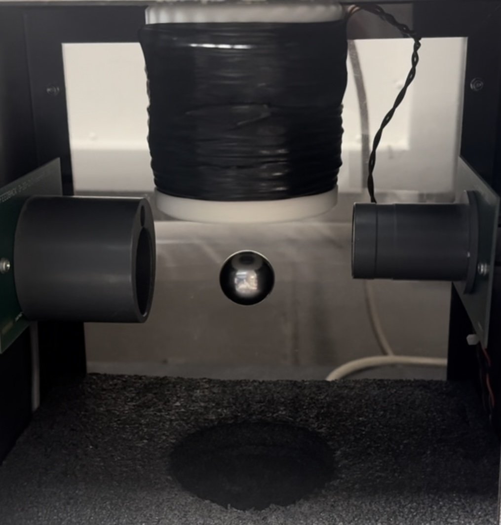
To better understand control systems, I worked with a team of 3 to create and analyze an electromagnetic levitation system using a PID controller. The controller had to operate at multiple settings: pure levitation, square wave input, sinusoidal input, and random input. The majority of this project was done using LabVIEW and NI Data Acquisition.
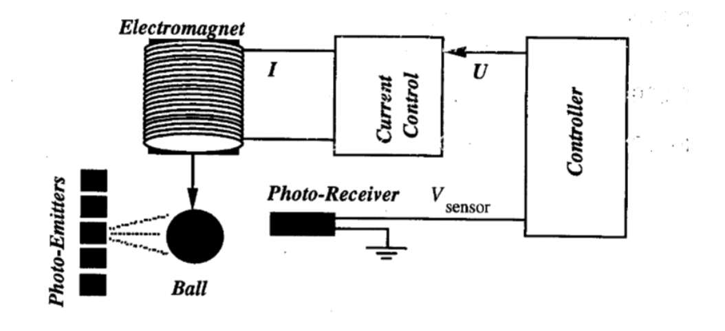
Schematic of MagLev system. Taken from chapter 2 of Feedback® Instruments Ltd Magnetic Levitation System Manual Supplement (2023).

Theoretical block diagram of system
The MagLev system levitates a metal ball using an electromagnet (above the ball) and a position sensor that outputs voltage signals corresponding to the ball’s height. Using a PID controller, the MagLev reads the position of the ball, compares it to desired height, then adjusts voltage to correct positional error. The PID has three nonzero values that we adjusted to attain precise levitation: proportional gain, Kp (adjusts intensity of magnet), time derivative, Td (adds damping force), and integral time, Ti (corrects error in voltage).
Analysis & MatLAB
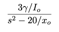
To tune our system, we began by finding a starting value for Kp. This was done by analyzing the general transfer function for the MagLev system:
To determine the transfer function for our specific system, we found γ and x₀ values using position vs height data (taken using DAQ Assist). γ is the inverse of height vs voltage slope, while x₀ is the intercept at which V=0 (measured from the top, so x₀= height to top of magnet - y-intercept). The graph of this data is shown below, and yields a γ value of 3.225 and an x₀ value of 3.96 cm. Finally, current was solved for using Ohm’s law, and found to be .623 Amps.
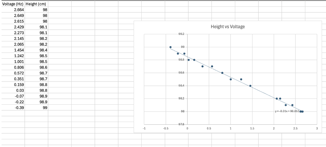
Height vs Voltage graph and line of best fit.
Thus, the transfer function for our specific system is as follows:
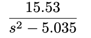
This transfer function was input into MatLAB’s SISO tool, generating the following plots and equations (Kp=1.5042):
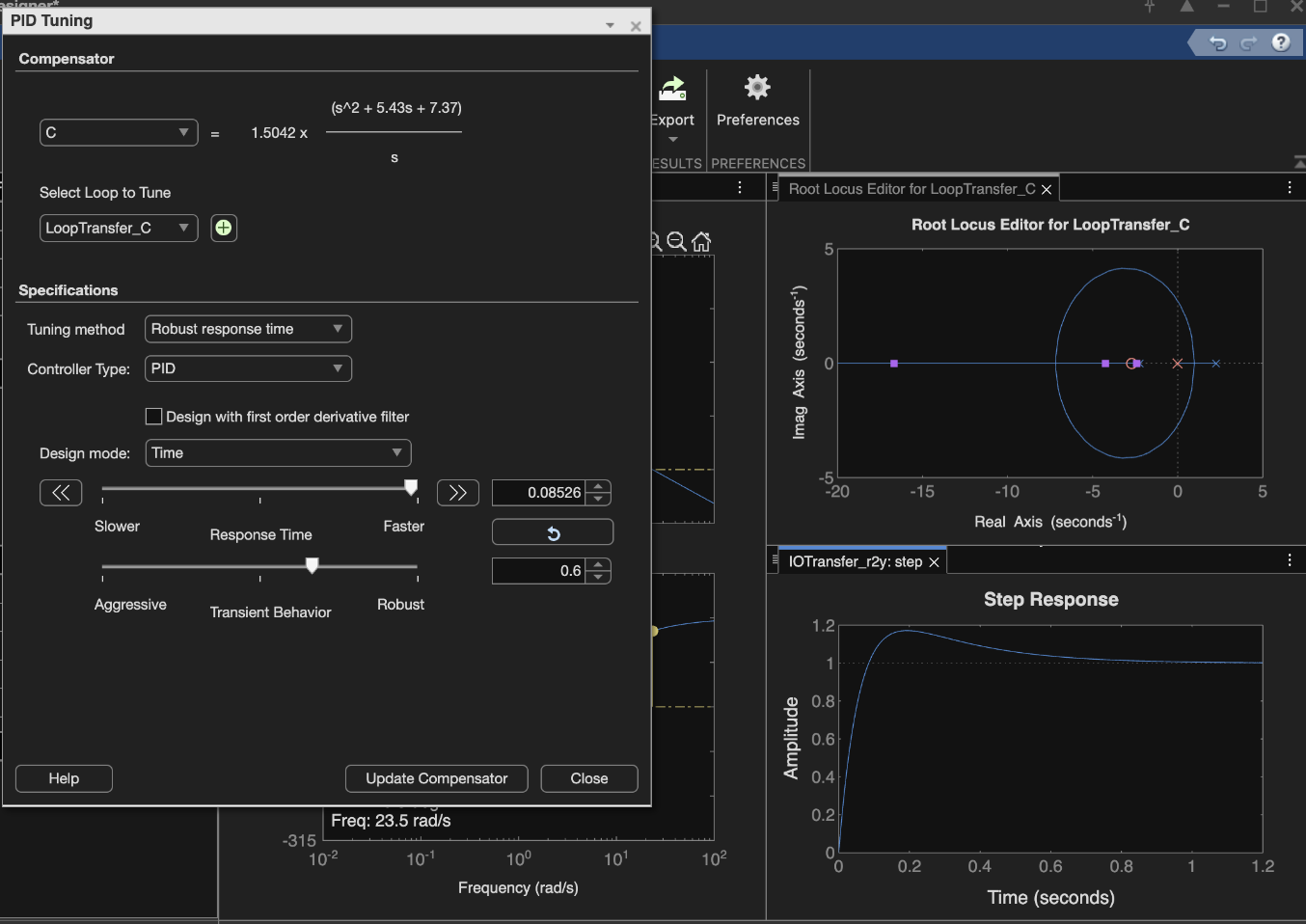
MatLAB SISO tool plots and PID Tuning. With specific transfer function input, and fast response selected, Kp=1.5042.
To begin tuning our Kp, Td, Ti values, we built the following LabVIEW system.
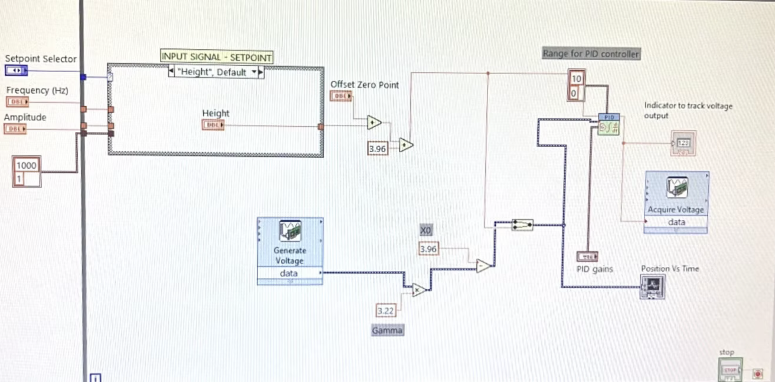
LabVIEW interface
After making the LabView interface shown below, we were able to find the best values for our PID controller. We found Kp to be between 1.5 and 1.6, Ti = 0.04, and Td=0.0004. These values worked for all user inputs and kept the error relatively small on our position graphs. For our sin waves, we found the ball to be most stable when Kp was 1.35, Ti was 0.04, and Td was 0.000444. With a height of 2, an amplitude of 0.5, and a frequency with 5 Hz, we get a stable sin wave. We also found that the ball still floats when the Kp value is between 1.5 and 1.6 and the frequency can be anywhere from 2-20 Hz.
Through the design process, we also got a better understanding of how the gain controller worked. The proportional gain controlled the strength of the magnet. To start tuning the controller, we first isolated Kp. Once we felt the ball begin to lift off our fingers, we knew the gain was strong enough to hold the ball in place. After that, we introduced derivative time, which helps reduce the error by damping the system. This allowed the ball to stay closer to its desired position.
Finally, we added integral time, which controls how quickly the system responds to error. When Td was too small, we saw more overshoot, but if it was too large, the controller became overly sensitive to sudden changes. We also continued tuning the rest of the inputs by slowly increasing the amplitude of the input. Once we reached a steady and stable response, we tested how much we could change the frequency before the ball dropped.
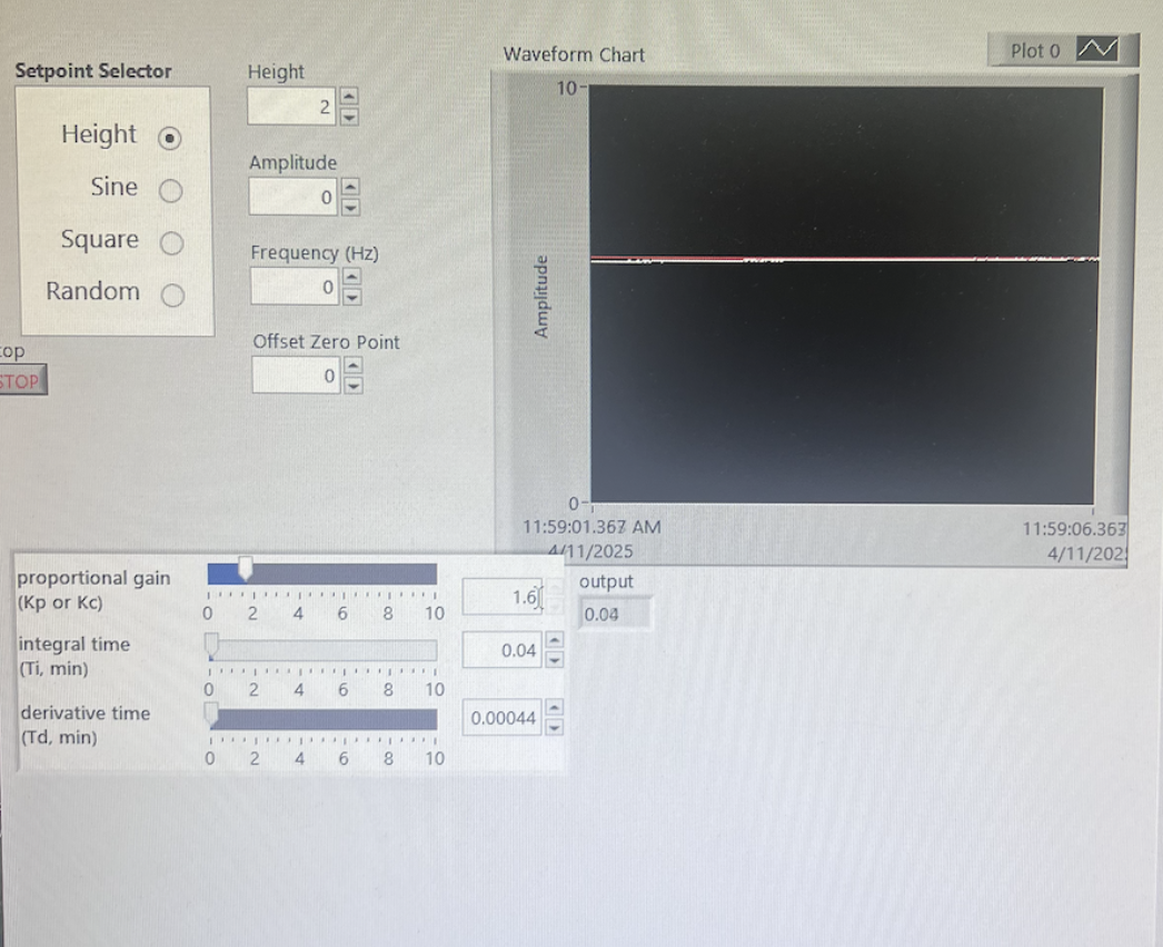
Waveform chart for constant height input
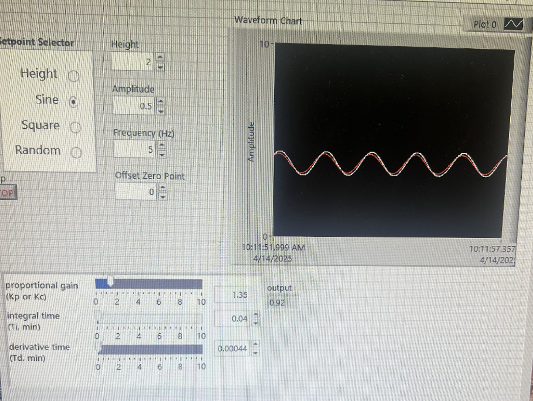
Waveform chart for sinusoidal input
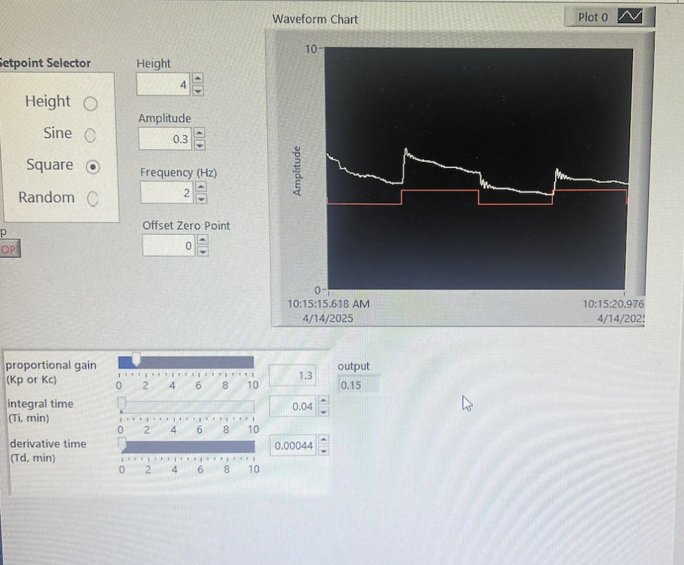
Waveform chart for square wave input
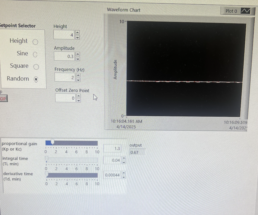
Waveform chart for random input